McXtrace homepage

Using simulation front-ends

5.4 Using simulation front-ends

McXtrace includes a number of front-end programs that extend the functionality of the simulations. A front-end program is an interface between the user and the simulations, running the simulations and presenting the output in various ways to the user.

The list of available McXtrace front-end programs is (see mxdoc --tools, or run any tool with -h for its speciﬁc help):

1    McXtrace Tools 
2       mcxtrace         Main instrument compiler 
3       mcxtrace-pygen  Alternative code generator: McStasScript Python model 
4       mxrun          Instrument build and execution utility 
5       mcxtrace-jupylab Opens a generated instrument model in JupyterLab 
6       mxgui          Graphical User Interface instrument builder 
7       mxdoc          Component library documentation generator/viewer 
8       mxplot         Simulation result viewer (default: pyqtgraph backend) 
9       mxplot-html     Simulation result viewer, in a web browser (D3.js) 
10       mxplotdiff-html Difference plot between two simulation results, in a browser 
11       mxcoplot-html   Overlay (co-plot) of two simulation results’ 1D monitors 
12       mxdisplay       Instrument geometry viewer (default: pyqtgraph backend) 
13       mxtest         Self-test / benchmark of the current McXtrace installation 
14       mxviewtest      Viewer for mxtest results, with mxplotdiff-html comparisons 
15    Each tool also exists in dedicated *-matplotlib, *-pyqtgraph, *-html, 
16    *-webgl or *-webgl-classic variants where applicable, see sections below. 
17    DOC:      Please visit https://www.mcxtrace.org

5.4.1 The graphical user interface (mxgui)

The front-end mxgui provides a graphical user interface that interfaces the various parts of the McXtrace package. It may be started with the single command

1    mxgui

The mxgui program may optionally be given the name of the instrument ﬁle to use.

Dependencies: As of McXtrace 3.x, mxgui is a pure Python/Qt application (PyQt), bundled with the standard conda-forge McXtrace package; no separate Perl, Tk, or PGPLOT installation is required.

The menus

When the front-end is started the main window is opened (see ﬁgure 5.1). This window displays the output from compiling and running simulations, and contains a few menus and buttons for easy navigation. The main purpose of the front-end is to edit and compile instrument deﬁnitions, run the simulations, and visualize the results.

The File menu has the following features:

File/Open instrument

selects the name of an instrument ﬁle to be used.

File/Edit current

opens a simple editor window with McXtrace syntax highlighting for editing the current instrument deﬁnition. This function is also available from the Edit button to the right of the name of the instrument deﬁnition in the main window.

File/Spawn editor

This starts the editor deﬁned in the environment variable VISUAL or EDITOR on the current instrument ﬁle. It is also possible to start an external editor manually; in any case mxgui will recompile instrument deﬁnitions as necessary based on the modiﬁcation dates of the ﬁles on the disk.

File/Compile instrument

forces a recompile of the instrument deﬁnition, regardless of ﬁle dates. This is for example useful to pick up changes in component deﬁnitions, which the front-end will not notice automatically. This might also be required when choosing MPI and NeXus options.

File/Save log ﬁle

saves the text in the window showing output of compilations and simulations into a ﬁle.

File/Clear output

erases all text in the window showing output of compilations and simulations.

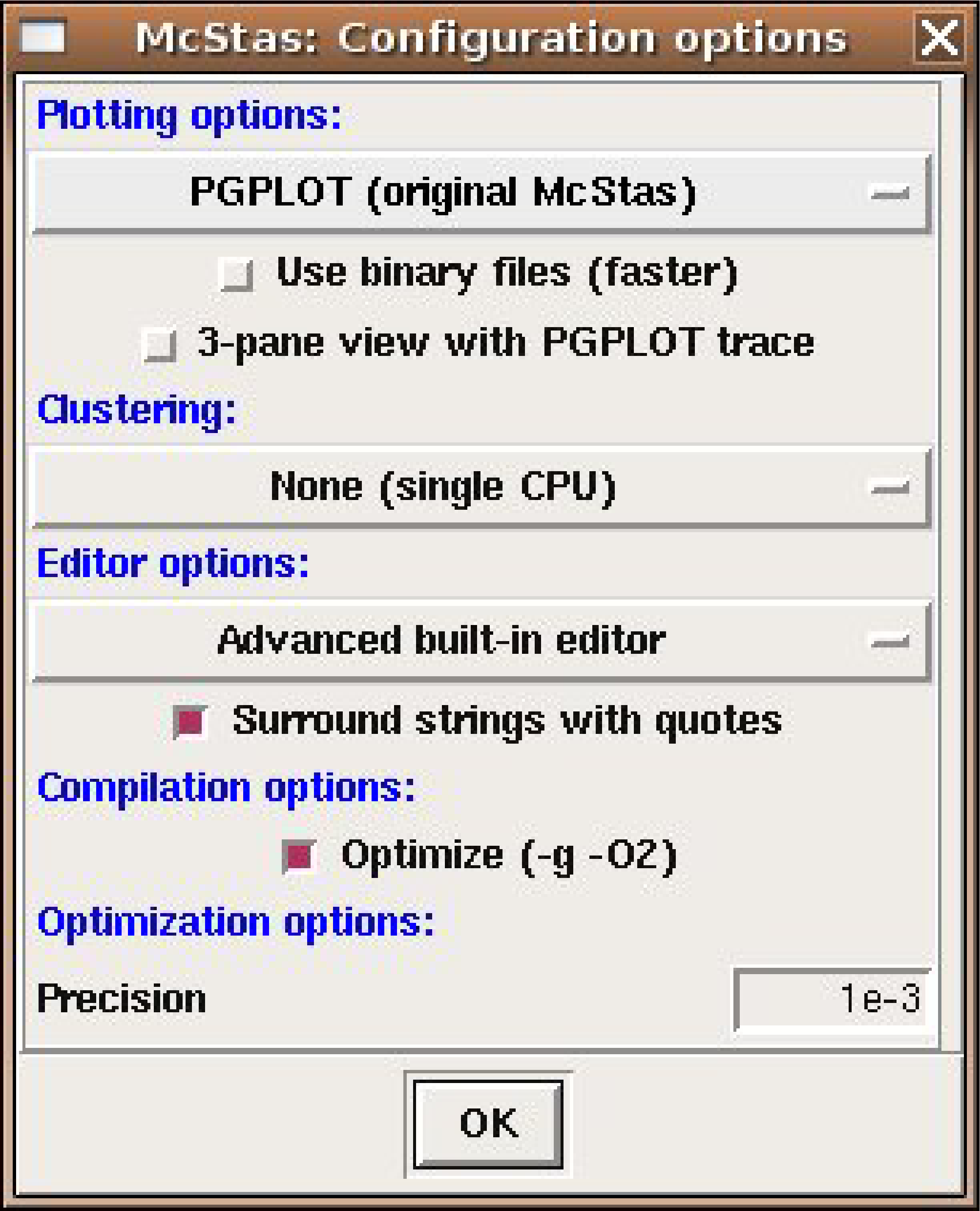
File/Preferences

Opens the conﬁguration dialog shown in ﬁgure 5.2. Several settings can be chosen here:

Selection of the desired plotting/display backend (pyqtgraph, matplotlib, html, …) for mxplot and mxdisplay.
Choice of code generator (mccode or mccode-antlr, see section 5.2.1.0).
Choice of editor to use when editing instrument ﬁles.
Automatic quotation of strings when inserting in the built-in editor.
Possibility to not optimize when compiling the generated c-code. This is very handy when setting up an instrument model, which requires regular compilations.

To save the chosen settings for your next McXtrace run, use Save Conﬁguration in the File menu.

File/Save conﬁguration

saves user settings from Conﬁguration options and Run dialogue to disk.

File/Quit

exits the graphical user interface front-end.

The Simulation menu has the following features:

Simulation/Read old simulation: prompts for the name of a ﬁle from a previous run of a McXtrace simulation (usually called mccode.sim). The ﬁle will be read and any detector data plotted using the mxplot front-end. The parameters used in the simulation will also be made the defaults for the next simulation run. This function is also available using the “Read” button to the right of the name of the current simulation data.
Simulation/Run simulation: opens the run dialog window, explained further below.
Simulation/Plot results: plots (using mxplot) the results of the last simulation run or spawns a load dialogue to load a set of results.

Figure 5.2.:

The “conﬁguration options” dialog in mxgui.

The New from Template menu (known as “X-ray Site” in older McXtrace releases) contains a list of template and example instruments as found in the McXtrace library, sorted by category/facility (e.g. Templates, ILL, ISIS, ESS, Union_demos, …). When selecting one of these, a local copy of the instrument description is transferred to the active directory (so that users have modiﬁcation rights) and loaded. One may then view its source (Edit) and use it directly for simulations/trace (3D View).

The Tools menu gathers minor tools.

Tools/Plot current/other results: Plot current simulation results and other results.
Tools/Dataset convert/merge: Opens a GUI to merge scattered data sets (e.g. from successive runs or an MPI job) or assemble scan sets.
Tools/Shortcut keys: displays the shortcut keys used for running and editing instruments.

The Help menu has the following features, through use of mxdoc and a web browser. To customize the used web browser, set the BROWSER environment variable. If BROWSER is not set, mxgui uses netscape/mozilla/firefox on Unix/Linux and the default browser on Windows.

Help/McXtrace User manual: calls mxdoc --manual, brings up the local pdf version of this manual, using a web browser.
Help/McXtrace Component manual: calls mxdoc --comps, brings up the local pdf version of the component manual, using a web browser.
Help/Component library index: displays the component documentation using the component index.html index ﬁle.
Help/McXtrace web page: calls mxdoc --web, brings up the McXtrace website in a web browser.
Help/Tutorial: opens the McXtrace tutorial for a quick start.
Help/Current instrument info: generates a description web-page of the current edited instrument.
Help/Test McXtrace installation: launches mxtest to check that the McXtrace package is installed properly and generates accurate results (see section 5.4).
Help/Generate component index: (re-)generates locally the component index.html.

The run dialog

Figure 5.3.:

The run dialog in mxgui.

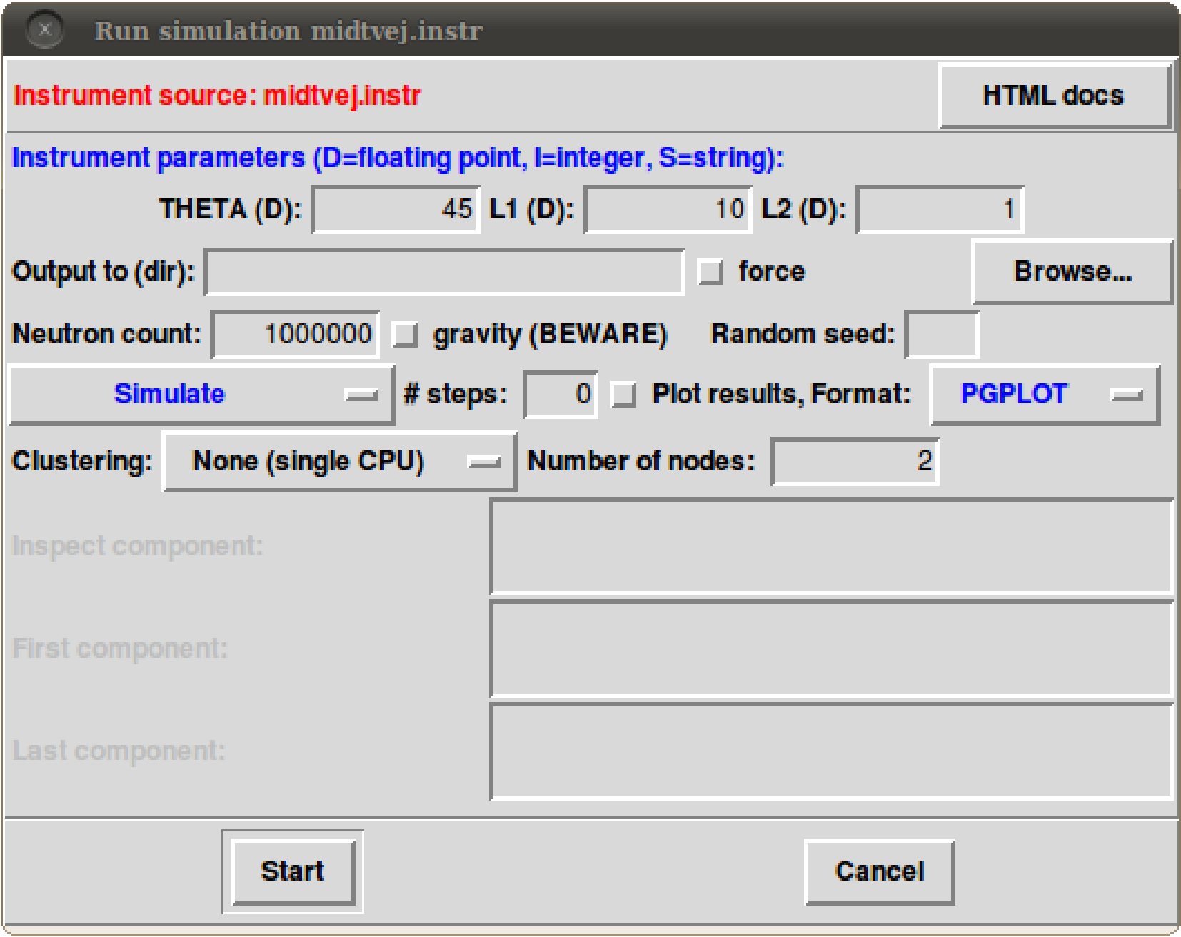
The run dialog is used to run simulations. It allows the entry of instrument parameters as well as the speciﬁcations of options for running the simulation (see section 5.3 for details). It also allows to run the mxdisplay (section 5.4.5) and mxplot (section 5.4.6) front-ends together with the simulation.

The meaning of the diﬀerent ﬁelds is as follows:

Run:Instrument parameters

allows the setting of the values for the input parameters of the instrument. The type of each instrument parameter is given in parenthesis after each name. Floating point numbers are denoted by (D) (for the C type “double”), (I) denotes integer parameters, and (S) denotes strings. For parameter scans and optimizations, enter the minimum and maximum values to scan/optimize, separated by a comma, e.g. 1,10 and do not forget to set the # Scanpoints to more than 1.

Run:Output to

allows the entry of a directory for storage of the resulting data ﬁles in (like the --dir option). If no name is given, the results are stored in the current directory, to be overwritten by the next simulation.

Run:Force

Forces McXtrace to overwrite existing data ﬁles

Photon count

sets the number of x-rays to simulate (the --ncount option).

Run:Gravity

Activates gravitation handling. Not all components full support the use of gravitation, but all transport in “free space” using the PROP_DT, PROP_Z0 etc. macros will include propagation with gravity. Only local, internal component propagation without the PROP routines will be gravity-less. As a conclusion it is considered safe and to high precision correct to apply the gravitation setting if one takes care to use the Guide_gravity component and other gravity-supporting guide types in combination with non-gravity components that are “small” in size, i.e. samples, lenses, etc.

Run:Random seed/Set seed to

selects between using a random seed (diﬀerent in each simulation) for the random number generator, or using a ﬁxed seed (to reproduce results for debugging).

Run:Simulate/Trace (3D)/Optimize

selects between several modes of running the simulation:

Simulate: perform a normal simulation or a scan when #steps is set to non-zero value
Trace (3D view): View the instrument in 3D tracing individual x-rays through the instrument
Optimize: ﬁnd the optimum value of the simulation parameters in the given ranges (see section 5.3.5).
Backgrounding (bg): Simulate or Optimize in the background.

Run:# steps / # optim

sets the number of simulation to run when performing a parameter scan or the number of iterations to perform in optimization mode.

Run:Plot results

– if checked, the mxplot front-end will be run after the simulation has ﬁnished, and the plot dialog will appear (see below).

Run:Format

quick selection of output format (McCode or NeXus).

Run:Clustering method

selects between running locally or via MPI. See section 5.6 on parallel computing for more informations.

Run:Number of nodes

sets the number of MPI nodes to use.

Run:Inspect component

(Trace mode) will trace only x-ray trajectories that reach a given component (e.g. sample or detector).

Run:First component

(Trace mode) seletcs the ﬁrst component to plot (default is ﬁrst) in order to deﬁne a region of interest.

Run:Last component

(Trace mode) seletcs the last component to plot (default is ﬁrst) in order to deﬁne a region of interest.

Run:Maximize monitor

(Optimization mode) seletcs up to three monitors which integral value should be maximized, varying instrument parameters. If no monitor is selected, the sum of all monitors is optimized.

Run:Start

runs the simulation.

Run:Cancel

aborts the dialog.

Most of the settings on the run dialog can be saved for your next McXtrace run using ’Save conﬁguration’ in the File menu.

Before running the simulation, the instrument deﬁnition is automatically compiled if it is newer than the generated C ﬁle (or if the C ﬁle is newer than the executable). The executable is assumed to have a .out suﬃx in the ﬁlename. NB: If components are changed, automatic compilation is not performed. Instead, use the File/Compile menu item in mxgui.

The editor window

The editor window provides a simple editor for creating and modifying instrument deﬁnitions. Apart from the usual editor functions, the “Insert” menu provides some functions that aid in the construction of the instrument deﬁnitions:

Editor Insert/Instrument template

inserts the text for a simple instrument skeleton in the editor window.

Editor Insert/Component…

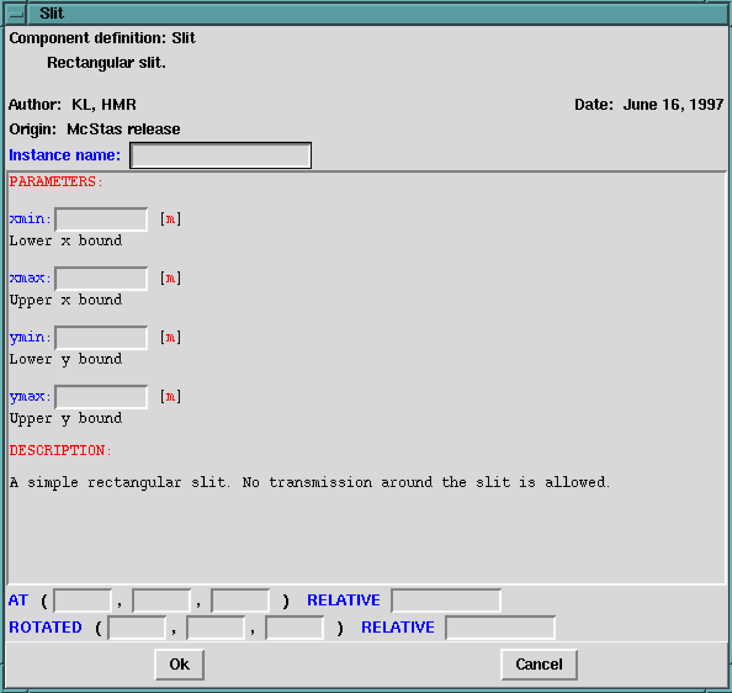
opens up a dialog window with a list of all the components available for use in McXtrace. Selecting a component will display a description. Double-clicking will open up a dialog window allowing the entry of the values of all the parameters for the component (ﬁgure 5.4). See section 6.3 for details of the meaning of the diﬀerent ﬁelds.

The dialog will also pick up those of the users own components that are present in the current directory when mxgui is started. See section 6.7 for how to write components to integrate well with this facility.

Editor Insert/Type

These menu entries give quick access to the entry dialog for the various component types available, i.e. Sources, Optics, Samples, Monitors, Misc, Contrib and Obsolete.

Figure 5.4.:

Component parameter entry dialog.

5.4.2 Running simulations on the commandline (mxrun)

The mxrun front-end provides a convenient command-line interface for running simulations with the same automatic compilation features available in the mxgui front-end. It also provides a facility for running a series of simulations while varying an input parameter.

The command

1mxrun sim args ...
 
2

will compile the instrument deﬁnition sim.instr (if necessary) into an executable simulation sim.out. It will then run sim.out, passing the argument list args

The possible arguments are the same as those accepted by the simulations themselves as described in section 5.3, with the following extensions:

The -c or --force-compile option may be used to force the recompilation of the instrument deﬁnition, regardless of ﬁle dates. This may be needed in case any component deﬁnitions are changed (in which case mxrun does not automatically recompile), or if a new version of McXtrace has been installed.
The -p file or --param=file option may be used to specify a ﬁle containing assignment of values to the input parameters of the instrument deﬁnition. The ﬁle should consist of speciﬁcations of the form name=value separated by spaces or line breaks. Multiple -p options may be given together with direct parameter speciﬁcations on the command line. If a parameter is assigned multiple times, later assignments override previous ones.
The -N count or --numpoints=count option may be used to perform a series of count simulations while varying one or more parameters within speciﬁed intervals. Such a series of simulations is called a scan. To specify an interval for a parameter X, it should be assigned two values separated by a comma. For example, the command
```
1mxrun sim.instr -N4 X=2,8 Y=1
      
2
```
would run the simulation deﬁned in sim.instr four times, with X having the values 2, 4, 6, and 8, respectively.
After running the simulation, the results will be written to the ﬁle mccode.dat by default (see the --optimise-file option). This ﬁle contains one line for each simulation run giving the values of the scanned input variables along with the integrated intensity and estimated error in all monitors. This ﬁle can be plotted with any of the mxplot backends, see section 5.4.6.
When performing a scan, the --optimise-file file option makes mxrun write the scan summary to ﬁle instead of the default mccode.dat.
Two further scan modes are available besides the default one, in which all scanned parameters step together from their minimum to their maximum value. With -M or --multi, the cartesian product of all scanned parameters’ points is run (a multi-dimensional “grid” scan); the point count of each parameter is then given as a comma-separated list to -N, in the order the parameters appear on the command line. For example
```
1mxrun sim.instr -M -N3,5 X=2,8 Y=0,1
      
2
```
runs \(3\times 5=15\) simulations. With -L or --list, each scanned parameter is instead given as an explicit comma-separated list of values (which also allows non-numerical values such as ﬁle names); lists of equal length are stepped through together, and combined with -M the cartesian product is run (the lists may then have diﬀerent lengths). A parameter may also be given as min:delta:max , in which case the point count follows from the requested step size and the parameter may be freely mixed with explicit lists. The option --seeds scans over a range of random seeds (each non-zero).
With --autoplot, mxrun opens a plotter on the generated data set when done (the back-end is chosen with --autoplotter, and --invcanvas requests an inverted canvas). With -C or --c-lint, the generated C code is only passed through a C linter (e.g. cppcheck, conﬁgured in mccode_config.json) and no simulation is run.
When performing a scan, the -d dir and --dir=dir options make mxrun put all output in a newly created directory dir. Additionally, the directory will have subdirectories 1, 2, 3,…containing all data ﬁles output from the diﬀerent simulations. When the -d option is not used, no data ﬁles are written from the individual simulations (in order to save disk space).

The -h option will list valid options; see also Table 5.1 for the complete, current option list.

5.4.3 Interactive notebooks (mcxtrace-jupylab)

The mcxtrace-jupylab front-end oﬀers an interactive, notebook-based alternative to editing an .instr ﬁle directly and running it via mxgui/mxrun. Given an instrument ﬁle:

1mcxtrace-jupylab name.instr

it ﬁrst runs mcxtrace-pygen (see above) to translate the instrument into an equivalent McStasScript Python model, writes that model into a notebook (name_generated.ipynb) built from a ready-made template (imports, and cells calling show_diagram(), show_instrument(), backengine() and the plotting helpers are already ﬁlled in), and opens it in JupyterLab¹ . From there the instrument can be inspected, modiﬁed and run cell by cell using McStasScript’s own Python API, which is useful for exploratory work and for combining a simulation with other Python-based analysis in the same notebook.

Note that this generates a McStasScript model once, as a starting point; it is not kept in sync with later edits to the original .instr ﬁle, nor vice versa. See the McStasScript documentation [Mcs] for the Python API itself.

5.4.4 GPU acceleration via OpenACC

McXtrace 3.x supports GPU-accelerated simulations through the OpenACC framework, enabling substantial speed-ups over CPU-only execution on compatible NVIDIA hardware.

Requirements

Compiler: NVIDIA HPC SDK version 20.x or newer. The free Community Edition is suﬃcient.
Hardware: A CUDA-capable NVIDIA GPU with an up-to-date driver.
Platform: GPU support is currently available on Linux only. Windows is not yet supported for OpenACC by NVIDIA; Windows users wishing to use GPU acceleration should do so via WSL 2 running a Linux distribution.

Running a GPU-accelerated simulation

Pass the --openacc ﬂag to mxrun:

  mxrun --openacc MyInstrument.instr -n 1e9

The OpenACC execution can be tuned with --vecsize (vector length), --numgangs (number of “gangs”), --gpu_innerloop (maximum number of particles per GPU kernel run; if smaller than the requested x-ray count, the kernel is repeated) and --funnel (funnelled simulation ﬂow, e.g. for mixed CPU/GPU execution), see Table 5.2 and Table 5.1.

Combined multi-core + GPU execution. It is also possible to use both CPU cores and the GPU simultaneously. Enable this by adding the following to the OACCFLAGS ﬁeld of your mccode_config.json:

  "OACCFLAGS": "-fast -Minfo=accel -acc=gpu,multicore
                -gpu=managed -DOPENACC -DMULTICORE"

Further information

GPU terminology speciﬁc to McStas/McXtrace 3 and detailed debugging tips are documented on the McCode wiki:

GPU terminology table:
https://github.com/mccode-dev/McCode/wiki/McStas-McXtrace-3-and-GPU-terminology-(table)
GPU debugging tips:
https://github.com/mccode-dev/McCode/wiki/GPU-Debugging-tips

5.4.5 Graphical display of simulations (mxdisplay)

The front-end mxdisplay is a graphical visualization tool, very useful for debugging. It presents a schematic drawing of the instrument deﬁnition, showing the position of the components and the paths of the simulated x-rays through the instrument. It is thus very useful for debugging a simulation, for example to spot components in the wrong position or to ﬁnd out where x-rays are getting lost.

To use the mxdisplay front-end with a simulation, run it as follows:

1mxdisplay sim args ...
 
2

where sim is the name of either the instrument source sim.instr or the simulation program sim.out generated by mcxtrace, and args … are the normal command line arguments for the simulation, as explained above. The -h option will list valid options.

The drawing back-end may be selected by invoking one of the dedicated front-ends directly:

mxdisplay-pyqtgraph (the default when running plain mxdisplay): interactive PyQtGraph 3D view.
mxdisplay-matplotlib: static/interactive matplotlib 3D view. This is a thin wrapper script, so its options diﬀer slightly from the default front-end: --trace={1,2} selects the classic (1) or new (2, default) drawing mode, --backend=NAME selects the matplotlib back-end (the hard-copy back-ends pdf, pgf, ps and svg save a ﬁle instead of opening a window), and the number of traced rays is capped at 100.
mxdisplay-webgl and mxdisplay-webgl-classic: browser-based WebGL views (the former uses a small NodeJS-backed server for larger instruments/particle counts; its ﬁrst use performs a one-time npm/vite module installation, which needs internet access). In addition to the options listed below they accept -t/--trace N (visualisation mode, default 2 resp. 1), -d/--dirname DIR, --first COMP and --last COMP (the ﬁrst and last component of the zoomed range), and --nobrowse (do not open a browser); mxdisplay-webgl also has --timeout SEC (the shutdown time of its development server, default 300 s).
mxdisplay-cad: exports the instrument geometry to a CAD ﬁle and requires the cadquery Python package. The format is selected with -f/--format: step (default), stl, xml, vrml, gltf or vtkjs. As no rays are needed for a geometry export, --ncount defaults to 0 here.
mxdisplay-mantid_xml: exports an approximate Mantid Instrument Deﬁnition File (IDF) describing the detector geometry.

For instance, calling

1mxdisplay-webgl ./Template_1Slit_Diff.out SLITW=5e-6
 
2

will open a WebGL view of the instrument in a browser tab. The mxdisplay front-end can also be run from the mxgui front-end.

The (default, PyQtGraph) front-end accepts the following options, amongst others – run mxdisplay --help for the complete, current list:

--default: automatically use the instrument’s default parameter values, without prompting.
--dirname=DIR: override the output directory name used while tracing.
--inspect=comp: only display x-ray trajectories that reach the component named comp. This is useful when debugging, e.g. to hide x-rays absorbed upstream of the component of interest.
--invcanvas: invert the canvas background from black to white (useful for printing or screenshots).
-n/--ncount=N: number of x-rays to trace (default 300).
--no-mpi: simulate without MPI (forwards --no-mpi to mxrun).

All variants run mxrun --trace underneath, so an instrument parameter may be given as name=value just as for mxrun. In the PyQtGraph viewer, q quits, p saves a PNG image, s saves an SVG image (not on Windows), space or F5 shows the next ray, a click on a sub-plot zooms in on it (right-click to leave the zoomed view), and h or F1 lists the components. A legacy Matlab/Octave variant, mxdisplay-matlab, also exists under tools/matlab (it falls back to the Python mxdisplay when neither Matlab nor Octave is found).

When debugging trajectories through a long or complex instrument, combining --inspect with a modest --ncount typically gives the clearest, fastest picture of what is happening around a particular component.

5.4.6 Plotting the results of a simulation (mxplot)

The front-end mxplot is a program that produces plots of all the monitors in a simulation, and it is thus useful to get a quick overview of the simulation results.

In the simplest case, the front-end is run simply by typing

1    mxplot
 
2

This will plot any simulation data stored in the current directory, which is where simulations store their results by default. If the --dir option has been used (see section 5.3), the name of the ﬁle or directory should be passed to mxplot, e.g. “mxplot dir ” or “mxplot file ”. It is also possible to plot one single text (not binary) data ﬁle from a given monitor, passing its name to mxplot.

As with mxdisplay (section 5.4.5), the drawing back-end may be selected by invoking the dedicated front-end directly: mxplot-pyqtgraph (the default), mxplot-matplotlib, or mxplot-html (renders an interactive, self-contained web page using D3.js, see section 5.3.2), or by setting the MCXTRACE_FORMAT environment variable.

The back-ends share the simulation ﬁle or directory argument, and have a few options of their own. mxplot-html accepts -n/--nobrowse (do not open a browser), -l/--log (log scale), --autosize (expand the plots to the window size), -o/--output FILE (output .html ﬁle) and -W/-H (width and height of the plot frames). mxplot-matplotlib accepts --log, --backend NAME, --format FMT together with --output FILE (save as pdf, png, eps, svg, … without opening a window) and --html (save as HTML via mpld3; Linux only), and mxplot-pyqtgraph accepts --invcanvas (white instead of black canvas). Both the matplotlib and PyQtGraph variants also take -t/--test, which only runs the data loader and prints the structure of the plot. A legacy Matlab/Octave/iFit variant, mxplot-matlab, exists under tools/matlab; it picks whichever of Matlab, iFit and Octave is available (falling back to the Python mxplot), and can export each monitor with -png, -jpg, -fig, -eps or -pdf.

All plotters read the plain-text McXtrace/McCode data format (section 5.5); NeXus ﬁles are not currently read back by the plotters.

The mxplot front-end can also be run from the mxgui front-end.

The initial display shows plots for each detector in the simulation.

Comparing simulation results: mxplotdiﬀ and mxcoplot. Two companion tools share the loading and monitor-matching code of mxplot to compare simulation results (output directories, or single monitor ﬁles), matching monitors by output ﬁlename. Each exists in the same three rendering variants as mxplot (-html, -matplotlib and -pyqtgraph); the browser-based HTML variants are described here:

mxplotdiff-html a b plots, for every monitor present with matching binning in both a and b, the diﬀerence a - b (with error-propagated error bars for 1D monitors, and a diverging blue/white/red colour scale for 2D monitors). This is useful to quickly spot the eﬀect of a component or parameter change, an McXtrace version upgrade, or MPI vs. non-MPI results. By default, each diﬀerence is also written back out as a normal McXtrace/McCode-format data set (with an mccode.sim index), so the result directory can be reopened by any other McCode-format-aware plotter; pass -D/--no-dat to skip this. It always compares exactly two datasets.
mxcoplot-html a b [c ...] instead overlays the 1D monitors of two or more datasets on the same axes, for a direct visual comparison of curve shape and position (only 1D monitors are supported; a monitor that is not a matching 1D monitor in every dataset is skipped with a warning). The compact legend letters A, B, C, … are explained in an identity line under the title. Use -L/--labels A,B,C to set a short label per dataset, -C/--colours c1,c2,... to set the overlay colours, and --no-legends / --no-titles to leave out the on-plot legend respectively the in-plot title and identity line.

mxplotdiff-html accepts -A LABEL_A/-B LABEL_B to control the labels used for each input, and both tools accept -o OUTPUT to control the output directory name, -n/--nobrowse, -l/--log and --autosize; run either with --help for the complete option list. The matplotlib and PyQtGraph variants take the same dataset arguments and labelling options, plus the output options of the corresponding mxplot back-end. mxplotdiff-html and mxcoplot-html are also used internally by mxviewtest (section 5.4) to compare test runs against a reference.

5.4.7 Creating and viewing the library, component/instrument help and Manuals (mxdoc)

McXtrace provides an easy way to generate automatically an HTML help page about a given component or instrument, or the whole McXtrace library.

1mxdoc 
2mxdoc searchterm 
3mxdoc file.comp

The ﬁrst example generates an index.html catalog ﬁle using the available components and instruments (both locally, and in the McXtrace library), and browses it using the BROWSER environment variable (e.g. ﬁrefox, chromium, …). Alternatively, if a search term or a ﬁle.comp/ﬁle.instr path is given, mxdoc will search within the library and open documentation for all matching entries.

Additional options include --install/-i (regenerate the local installation-wide index), --dir=DIR/-d (add search results from a given directory), and --verbose/-v (print a parsing log). HTML is always written; --md/-M and --tex/-T also emit Markdown respectively LaTeX documentation ﬁles (--all-formats/-A for all three) — the LaTeX snippets of the component library that make up the Component Manual are produced this way. With --in-repo the output is placed next to the source ﬁles instead of in the installed documentation directory (and no master page is made), and --outdir=DIR/-o selects the output directory (in-repo use only). The options --manual/-m, --comps/-c and --web/-w will open the User Manual (this document), the Component Manual, and the McXtrace web site, respectively, all requiring BROWSER to be deﬁned. Finally, the --help option will display the command help, as usual.

See section 6.7 for more details about the McDoc usage and header format. mxdoc is a pure Python tool, part of the standard McXtrace conda-forge package.

Online wiki. In addition to this manual, extensive and frequently updated documentation is maintained on the McCode GitHub wiki [Wik]:

https://github.com/mccode-dev/McCode/wiki

The wiki includes end-user guides, component development howtos, GPU acceleration information, and migration guides from McXtrace 2.x to 3.x.

5.4.8 Self-testing the installation (mxtest, mxviewtest)

McXtrace ships with a Python self-test/benchmark harness, replacing the earlier mxrun --test command. mxtest compiles and runs a selection (or all) of the example instruments found under the current installation(s), and stores each run’s results (including any test-deﬁned %Example reference values) in a timestamped output folder. Each test compiles the instrument, displays it with a single particle, runs it, and compares the result with the target value recorded in the instrument header. Useful options include --ncount (default \(10^6\)), --seed (default 1000; 0 randomizes), --mpi, --no-mpi, --openacc and --nexus (forwarded to mxrun for every tested instrument), --lint (only run the C linter, no simulations), --config=LABEL (test only a speciﬁc McCode installation/conﬁg), --instr=REGEX (test only matching instrument names), --comp=COMP[,COMP...] (test only instruments using any of the given components), --local=DIR (test instruments from DIR instead of the installation), --limit=N (test only the ﬁrst N instruments per version), --skipnontest (skip instruments without an %Example line), --strict (fail instruments without %Example line(s) immediately) and --permissive (exit with status 0 even if tests fail), --testdir=DIR and --suffix=SUFFIX (where the results are written), --compilemax, --runmax and --displaymax (time limits in seconds) and --noplots (do not generate the overview plots); run mxtest --help for the full list.

mxviewtest then generates an HTML report of one or more mxtest runs found in a given folder (the current directory by default). When more than one run is present (e.g. a reference run and a run on a diﬀerent platform, GPU vs. CPU, or a diﬀerent McXtrace branch), it takes the oldest subfolder as the reference column (override with --reflabel=LABEL), and additionally runs mxplotdiff-html and mxcoplot-html (section 5.4.6) between each other column’s monitor output and the reference’s, adding a DIFF [vs ref] link next to each such row in the report. These comparisons are cached on disk and generated in parallel (--diffworkers, each limited to --diffmax seconds), so re-running mxviewtest is fast; use --nodiff to skip generating them entirely, or --diff-errors-only to only diﬀ rows that already show a discrepancy (by default every valid row is diﬀed). --nobrowse keeps the ﬁnished report from being opened in a browser.